Modeling

A modeling assessment is one of a number of optional methods applied in site investigation and evaluation (Chapter 4). This chapter includes guidance on the use of PVI models and reporting of modeling results (Section 1.1); a summary of VI model types; steps in using the models and the reporting of results (Section 1.2); and, lastly, a discussion of the BioVapor Model (Section 1.3).

The discussion of specific model use is focused on the relatively simple PVI model BioVapor, a one-dimensional analytical model that includes aerobic biodegradation (DeVaull, McHugh, and Newberry 2009; API 2010), but also applies for the similar PVIScreen model (Weaver 2012). Other PVI models may also be appropriate for use; a list of models is included in Appendix H. Both BioVapor and PVIScreen are similar in concept to the broadly applied Johnson and Ettinger (J&E) model (Johnson and Ettinger 1991; USEPA 2009d), but, in addition, include the significant effects of aerobic biodegradation. The J&E model has been widely used for assessing the effects of contaminated vapors on indoor air, but is not recommended for evaluation of PVI because it does not include aerobic biodegradation (USEPA 2013a), and is therefore overly conservative.

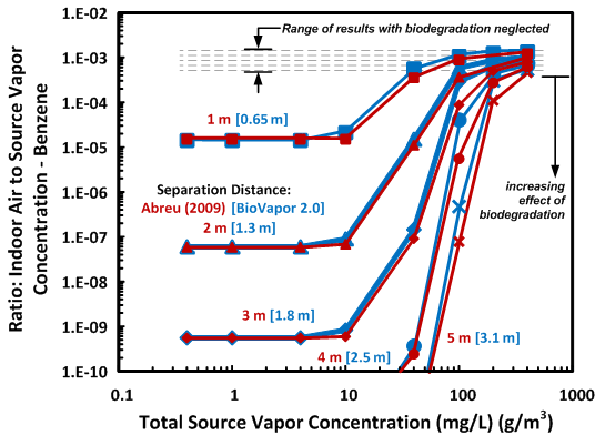
BioVapor and other models that incorporate biodegradation show distinct behavior for aerobically-degradable petroleum vapors. This behavior is illustrated in Figure 5-1, which includes model results for both BioVapor and a similarly-applied, three-dimensional numerical model (Abreu and Johnson 2006; Abreu, Ettinger, and McAlary 2009a; Abreu, Ettinger, and McAlary 2009b) in a typical basement scenario. Figure 5-1 shows the significant effects of biodegradation on benzene, both with increasing vertical building-source separation distance and with lower source vapor concentrations, as compared to results which neglect biodegradation. Modeling of other petroleum chemicals (not shown in Figure 5-1) exhibits results similar to Figure 5-1, but the precise estimates will vary.

Example model results illustrating the effects of biodegradation on chemical concentrations reaching indoor air. Significantly lower indoor air concentrations occur for both lower source vapor concentrations and at increased separation distance, as compared to model results which neglect biodegradation. Both three-dimensional (Abreu, Ettinger, and McAlary 2009b; API 2009) and BioVapor model results are shown in a typical basement scenario for benzene.

Another observation from Figure 5-1 is that the range of PVI scenarios can lead to high, transitional, and low ratios of indoor air to source vapor (indoor-to-source) concentration or attenuation factor. Three groups of site conditions and their potential for VI are evident:

At high source concentrations and short distances, high indoor-to-source concentration ratios are predicted, which may present potential concerns.
In the transitional range, small changes in site and scenario conditions and related parameters may significantly affect the indoor-to-source concentration ratios predicted and thus the potential for indoor VI.
At low source concentrations and greater distances, very low indoor-to-source ratios are predicted, indicating no potential concern or need for further evaluation of any kind (beyond delineation of a spill zone).

These scenarios illustrate the need for a sensitivity analysis when using VI models, particularly for model applications in the transitional range, for which small changes in input parameters may significantly change the potential for PVI. Sensitivity analysis is discussed in greater detail in Section 1.1.5 and, for the BioVapor model, in Section 1.3.2.

Use of Models for Assessing PVI

PVI models may be useful for sites that require further assessment based on the screening and application of the vertical screening distances described in Chapter 3, Site Screening. The complexity of modeling applications can vary greatly depending on the objectives of the modeling and availability of project-specific information. In general the steps indicated in Figure 5-2 should be followed and documented in the modeling report.

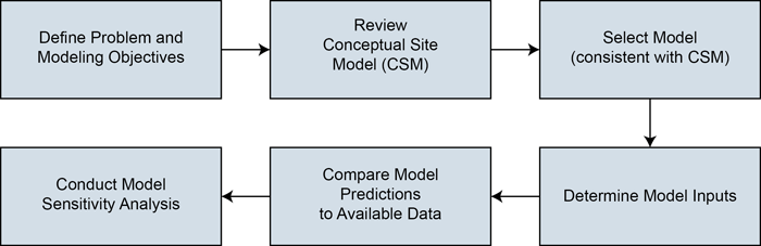
Steps in the modeling process.

Define the Problem and the Modeling Objectives

Prior to conducting any model simulations, the purpose and objectives of the modeling should be clearly understood and defined. The modeling objectives and purpose play a role in model selection. The objectives can also influence selection of parameter values and can help to determine the level of detail and accuracy required in the model simulations.

The following list includes example applications of PVI modeling, along with typical objectives for each modeling application:

Site-specific predictive modeling to assess current or future conditions. Modeling in this context is typically conducted in conjunction with a risk assessment. Input parameter values are selected to represent site conditions, but tend to be conservative because of the risk context. In some instances, such as where buildings do not currently exist but are planned for the future, modeling can predict vapor migration and attenuation for the future conditions anticipated at the site.
Site-specific modeling to help develop a CSM. PVI models can be used to explain key processes and data and to test and verify the CSM through comparison to available data. At petroleum release sites, a biodegradation model, such as BioVapor, may be used to match measured O₂ and PHC profiles in soil gas. Used in this way, a model can help to test and verify the CSM and evaluate the significance of vapor attenuation processes. In addition, PVI models can be used to evaluate the possible contribution of background sources to indoor air relative to the contribution from subsurface vapor sources.
Inverse modeling to develop site-specific cleanup goals. Some agencies may allow the derivation of site-specific cleanup goals through inverse modeling. With inverse modeling, acceptable concentrations of contaminants in indoor air are first identified. Then, a site-specific model is used to back-calculate the predicted concentrations needed in soil gas, soil, or groundwater to attain the acceptable contaminant concentrations in indoor air.
Remedial design and selection. A PVI model can be used to assess the O₂ flux to the subsurface that is required to achieve cleanup goals as part of a soil gas mitigation evaluation and technology selection process.
Modeling to support the development of PVI screening criteria and distances. Modeling in this context may be relevant or applicable when conditions or assumptions differ from those presented in Chapter 3. An example is a petroleum vapor source composition that differs significantly from gasoline. The screening criteria may include site-specific vertical screening distances or modified source-to-indoor air ratios, which apply when specific conditions are met.

For modeling, a tiered process is generally used. Initially, when site-specific data may be lacking, a model may rely on generic, conservative assumptions. Predictions at this tier are intentionally conservative and based on a simplified CSM, thus the model tends to overestimate exposure and risk. If site management decisions cannot be made at this stage, or the model estimates an unacceptable level of risk is present at this stage, then the modeling may progress to a refined tier, where some of the conservatism is addressed with additional site-specific data.

Review Conceptual Site Model

A model application should be consistent with the CSM developed for a site, summarizing the source of vapors, the expected migration pathways, important processes affecting vapor migration and attenuation, and the receptor that may be potentially exposed to the vapors. Clearly document components of the CSM and how they apply to the model. The CSM may contain areas of uncertainty because of a lack of field data. These areas of uncertainty and how they affect the modeling objectives should also be documented.

Select an Appropriate Model

An appropriate model should be selected to simulate the physical system defined in the CSM and for which site-specific data are available to populate the model. More complex models demand more input parameters, and the requirements for site-specific data collection increase with model complexity. It is critical that the model formulation and assumptions are consistent with site conditions and the CSM. For example, if the PVI source is not beneath the building, and depending on model objectives, selection of a one-dimensional upward transport model may not be appropriate.

Section 1.2 and Appendix H discuss models that incorporate biodegradation, and are thus appropriate for potential PVI sites. BioVapor is described in greater detail in Section 1.3.

The computer code selected for the modeling application should be well documented and have been tested for the intended use. A brief description of the model code should be provided in a report along with citations for model documentation.

Determine Model Inputs, Compare Model Predictions to Data, and Calibrate Model

In matching models to data, the ranges of model parameter values should be consistent with the CSM and based on empirical data. In model calibration, model estimates are compared to available data then, if they differ significantly, the model and the data are reevaluated, and the model inputs are adjusted as warranted. Typically, model comparisons focus on soil vapor data because indoor air may be affected by background sources of PHC chemicals.

Model calibration may or may not be part of the modeling application, depending on the modeling purpose, objectives, and available data. Where a model is not calibrated to field data, choose input parameter values that result in overestimates of concentrations and indoor exposure.

If a model is calibrated, then document the calibration criteria, procedure, and results, as well as the source and relevance of the observed data used in the calibration.

Conduct Model Sensitivity Analysis

Some degree of uncertainty is associated with predictive modeling results; understanding this uncertainty allows better interpretation of these results. Uncertainty can be assessed by performing a sensitivity analysis, which identifies those parameters that most significantly influence the modeling results.

Sensitivity analysis assesses the effect of parameter variation on model results and can be per- formed during model simulations and during model calibration. The reliability of the model can be assessed by evaluating the sensitivity of model responses to changes in parameter values that reflect plausible parameter uncertainty. The uncertainty may be bounded by selecting worst-case and best-case input values. Sensitivity analysis can also be performed to help identify data deficiencies.

Model applications should address the sensitivity of model outcomes to the choices made in the model inputs. Uncertain parameters that have a strong influence on model results should be identified and discussed. A notable example is the aerobic biodegradation rate, which can exert a significant influence on modeling results for a PVI site.

Parameter uncertainty and sensitivity analyses are critical components of any modeling exercise and are often recommended as best practices (USEPA 2004; ITRC 2007). These practices are especially valuable for screening assessments, in which model input parameters (such as pressure differential, soil permeability, ventilation rate, and moisture content) are not easily measured and are generally unknown for a specific site. The difficulty in obtaining measurements for some parameter inputs has forced investigators to rely heavily on literature values or professional judgment. To aid in selecting inputs, default parameter ranges and look-up tables have been defined (Johnson et al. 2002; Johnson 2005; USEPA 2004; Tillman and Weaver 2007). Where parameters are both uncertain and sensitive, it is generally best to choose conservative values.

Models for Petroleum Vapor Intrusion

The use of PVI models in regulatory programs varies, and continues to vary, as rules and regulations are revised. A recent U.S. state survey (MADEP 2010) indicates that, in states where VI modeling may be applied, it: (1) may be used as the sole basis for eliminating consideration of the VI pathway (11 states); (2) it may be applied as a line of evidence in the investigation (7 states), or (3) if applied, it may require confirmatory sampling (8 states).

Three types of models are used to evaluate PVI:

empirical models, which use predictions based on observations from other sites (such as bioattenuation factors)
analytical models, which are mathematical equations based on a simplification of site conditions (such as the J&E model)
numerical models, which allow for simulation of multidimensional transport and provide for more realistic representation of site conditions

This section provides an overview of PVI models that incorporate aerobic biodegradation, with additional details provided in Appendix H.

Empirical Models

Empirical models use an appropriate distance or attenuation factor derived from a compilation of relevant data to screen a site for PVI potential or to estimate an indoor air concentration. The vertical screening distances discussed in Chapter 3 are the result of empirical modeling.

Analytical Models

Analytical models for assessment of PVI exclusively consist of one-dimensional or compartmental models with a uniform planar subsurface source at a specified depth. A primary distinguishing feature of analytical models for PVI application is whether they incorporate biodegradation. A comparison of models for evaluation of VI both for CVOCs and for PHCs is presented in the Bekele study (Bekele et al. 2013).

The BioVapor model (DeVaull 2007; API 2010) is a modification of the J&E model incorporating O₂-limited biodegradation and includes improvements on earlier models (Johnson, Kemblowski, and Johnson 1998, 1999; Spence and Walden 2011). These improvements include options for setting several different boundary conditions for O₂ recharge to the subsurface, as well as accounting for all PHC present. The O₂-limited model only simulates biodegradation in soil zones when there is sufficient O₂, which is an important feature for biodegradation models. The BioVapor model has been extensively reviewed (Weaver 2012) and the USEPA is currently developing a version of this model (PVIScreen). The BioVapor model is described in greater detail later in this chapter.

Numerical Models

Numerical models offer potential advantages for simulation of conditions requiring additional detail, such as heterogeneity, geometric complexity, and temporal variability. PVI numerical models have typically been applied to obtain a more detailed understanding of causes and effects of vapor transport and attenuation (specific models are identified in Appendix H). Because of their complexity, numerical models require more data and effort (and therefore increased cost) than analytical models and thus, for practical applications, are rarely used.

BioVapor Model

The BioVapor model (DeVaull 2007; API 2010) is a one-dimensional model based on a CSM similar to the J&E model, but it includes aerobic biodegradation. The BioVapor model has been reviewed and accepted by USEPA (Weaver 2012) and is the basis for the USEPA PVIScreen model (2014a). Currently, BioVapor has been cited by a number of regulatory agencies and programs (for example USEPA OUST, California, Michigan, Illinois, and Australia). BioVapor evaluates O₂-limited aerobic biodegradation using an analytical solution to calculate the aerobic depth below ground surface. This calculation describes a shallow aerobic layer where first-order biodegradation occurs and a deeper anaerobic layer where biodegradation does not occur (see Figure 5.3). In the absence of biodegradation, the BioVapor model produces equivalent results to the J&E model.

The BioVapor model helps to assess the significance of data for groundwater, soil vapor, and soil, when PHC concentrations exceed applicable screening criteria. The BioVapor Model should not be used when LNAPL or contaminated groundwater is in contact with a building, or directly entering a building, because the model does not simulate these conditions. The conceptualization for the BioVapor model is based on constant, uniform contamination source, diffusion-dominated transport and a single, homogeneous soil layer. There are certain conditions outside of this conceptualization where BioVapor should generally not be used such as significant pressure-driven flow (for example, a landfill setting) or transport through preferential pathways (for example, sewers directly connecting an LNAPL source to a building). There may be other conditions where BioVapor may be applied conservatively or to portions of the site, such as heterogeneous soil layers or nonuniform contamination sources. For BioVapor, as for any model, consult the applicable regulatory agencies to determine whether the model results will be accepted.

Model Input Parameters

BioVapor (and PVIScreen) are conceptually similar to the broadly applied J&E model and share many similar (often identical) defined model parameters. Default values and applicable ranges for model input parameters, including the additional parameters specific to the BioVapor model are provided in Table 5-1, along with a qualitative description of the sensitivity of BioVapor model to input parameters. Other guidance on the selection of J&E model input parameters is also available (see Hers et al. 2003; USEPA 2004; Weaver and Tillman 2005; Johnson 2005).

Input parameters for the BioVapor model that affect biodegradation aspects of the model are:

O₂ supply beneath the building
chemical parameters and concentrations, including all PHC sources or degradation products with oxidative demand (such as methane)
chemical-specific, first-order biodegradation rate constants
baseline rate for O₂ respiration in soils
minimum O₂ for aerobic respiration
distance from bottom of building foundation to contamination source
type of building foundation (which affects the O₂-supply boundary condition)

Information on key input parameters for biodegradation modeling is provided below.

Relevant model parameters, ranges, and parameter sensitivities for the BioVapor model
Parameter	Default value	Normal range	Parameter sensitivity	Reference
Values for building parameters
Indoor mixing height, L_mix (cm)	244 (Residential) 300 (Commercial)	(-)	Low	USEPA 2004 ASTM 2000
Air exchange rate, ER (1/day)	6 (Residential) 12 (Commercial)	Min: 1.3	Moderate	USEPA 2004 ASHRAE 2004
Foundation thickness, L_crack (cm)	15	(-)	Low	USEPA 2004
Foundation area, A_b (cm²)	1.06E+6	(-)	Moderate	USEPA 2004
Foundation crack fraction, h (cm²-cracks/cm²-total)	3.77E-4	0–1	Low to moderate	USEPA 2004
Total porosity (soil-filled cracks), q_T,crack (cm³-void/cm³-soil)	1.00	0–1	Low	USEPA 2004
Water-filled porosity (soil-filled cracks) q_w,crack (cm³-void/cm³-soil)	0.00	0–1	Low	USEPA 2004
Airflow through foundation, Q_s (cm³-air/sec)	83	Min: 0	High	USEPA 2004
General comments – effect of building parameters on model results: relatively insensitive, unless biodegradation is negligible sensitive to airflow through foundation, Q_s, if O₂ in the subsurface (and therefore aerobic biodegradation) is limited residential: (single-family house, slab-on-grade); commercial: (small office or retail building, slab-on-grade)
Values for vadose zone parameters
Soil porosity, q_T (cm³-void/cm³-soil)	0.375	0.1 – 0.5	Low	USEPA 2004, Johnson 2005
Soil water content, q_w (cm³-water/cm³-soil)	0.054	0 – 0.5	High	USEPA 2004, Johnson 2005
Soil organic carbon fraction, f_oc (cm³/cm³-soil)	0.005	0.0001 – 0.1	See Baseline Respiration	Nominal
Soil density – bulk, r_s (g-soil/cm³-soil)	1.7	1.5 – 2	Low	ASTM 2000
Airflow through foundation, Q_s (cm³-air/sec)	83	(-)	High	Hers et al. 2003, USEPA 2004
Air flow underneath foundation, Q_f (cm³-air/sec)	(-)	≥ Qs	High	No Default
O₂ concentration below building, at soil surface (atmospheric, for dirt-floor, otherwise apply if measured below foundation)	Optional	0 – 21%	High
Aerobic depth, L_a (cm)	Optional	0 – L_T	High
Minimum O₂ concentration for aerobic biodegradation, O₂_-min	1%	0 – 1%	Low	DeVaull, 2007
Annual median soil temperature, T (°C)	10	0 – 30	Low	USEPA 2004
Baseline soil O₂ respiration rate, L_base (mg-O₂/g-soil-sec); function of f_oc	1.956E-7	Minimum: 0	Low to Moderate	DeVaull, 2007
Depth to source (from bottom of foundation), L_T (cm)	300	(-)	Moderate to high	None
First order aerobic biodegradation rates, k_w (1/sec)	Chemical-specific	See text	Moderate to High	DeVaull 2011
Generally, model results can be sensitive to: parameters affecting subsurface O₂: airflow (Q_s, Q_f); O₂ at soil surface; baseline O₂ demand (f_oc, L_base); and diffusion (q_T - q_w). parameters affecting degradation: kinetic degradation rates (k_w); depth to source (L_T); diffusion (q_T - q_w); and moisture (q_w)
Values for source zone parameters
Chemical-specific source vapor concentration (mg/m³)	Scenario-specific	0–100,000	Moderate	See text
Total source vapor concentration (mg /m³)	0.054	0–100,000	High	See text
Generally, model results can be sensitive to higher total source vapor concentrations, for which O₂ may be limited. Any source chemicals which may aerobically biodegrade contribute to total O₂ demand (including methane).
References: USEPA 2004. User’s Guide for Evaluating Subsurface Vapor Intrusion into Buildings, Table 9. February 22, 2004. Online at itrcweb.org/FileCabinet/GetFile?fileID=6921. ASTM 2000. ASTM E-2081-00: Standard Guide for Risk-Based Corrective Action. American Society for Testing and Materials, Philadelphia, PA. ASHRAE 2004. American Society of Heating, Refrigerating and Air-Conditioning Engineers (ASHRAE). 2004. Ventilation for acceptable indoor air quality. ASHRAE Standard 62.1-2004. DeVaull, G.E. 2007. "Indoor vapor intrusion with O₂-limited biodegradation for a subsurface gasoline source." Environ. Sci. Technol. 41: 3241-3248.

O₂ Supply Below Building

BioVapor has three options for identifying the O₂ supply or flux below the building foundation (see Figure 5-3).

Constant airflow rate is typically used for solid foundations (basement or slab-on-grade), where air flow is induced by stack effect (or other mechanisms causing building depressurization) or by the effect of wind on buildings.
Constant O₂ concentration at surface below the building applies to earthen-floor foundations or dirt-floor crawl spaces, or where subslab O₂ concentrations are measured
Fixed aerobic depth below grade applies when measurement data on this depth are available.

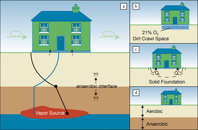
(a) BioVapor model biodegradation conceptualization; (b) O₂ boundary conditions consisting of constant O₂ concentration; (c) constant air flow; (d) fixed aerobic zone depth.

Source: Adapted from API (2011).

In the BioVapor model, two different airflow rates may be specified: airflow through the foundation (Q), and airflow under the foundation (Q_f). The Qs parameter relates solely to soil gas advection and is used to calculate the mass transfer of chemicals through the foundation as soil gas is drawn into a depressurized building. The Q parameter describes the advective airflow rate to below the foundation (Figure 5-3c), and is used solely for calculating the O₂ supply or flux into soil below the foundation that is available for aerobic biodegradation (based on airflow rate, assuming atmospheric O₂ concentration). Guidance on estimating the Qs parameter or soil gas advection rate, a common parameter for input into the J&E model, is provided in Hers et al. (2003) and USEPA (2004).

The BioVapor User’s Guide recommends that Q_f be assumed greater or equal to Q_s, because soil gas advection below and into the building also supplies O₂. In addition, O₂ mass flux by diffusion, both through the building foundation and through lateral migration from the sides of the building, will also supply O₂ for biodegradation. Modeling by DeVaull (2012) showed that when the foundation permeability is low (and thus the soil gas advection rate is low), the diffusive mass transport is proportionally high. In qualitative terms, this means that when Q_s is low, it generally is appropriate for Q_f to be higher than Q_s to account for O₂ diffusion.

Chemical Concentrations

The BioVapor model also requires information about PHCs. PHCs are a mixture of aliphatic and aromatic compounds (see Appendix C). Aliphatic compounds are composed of straight-chain, branched, or cyclic compounds and can be saturated (alkanes) or unsaturated (alkenes, alkynes, and others), whereas aromatic compounds contain one or more benzene or other conjugated heterocyclic rings within their structures. In general, aliphatic and aromatic hydrocarbons of moderate molecular weight (such as hexane or heptane) are more toxic than both lighter and heavier molecular weight aliphatic compounds commonly present at significant concentrations in soil vapors (USEPA 2009b). Aliphatic hydrocarbons are the primary components in vapors near petroleum sources such as gasoline and diesel.

The BioVapor model requires input of chemical concentrations for three groups of PHCs:

risk drivers (such as BTEX or hexane)
other PHC compounds, which are not risk drivers but represent an oxygen demand
hydrocarbon surrogates, which include multiple chemicals (for example, hydrocarbon ranges) and which may also not be risk drivers, but represent an oxygen demand

Contaminant concentrations for both soil gas or groundwater sources may be entered, and new chemicals may be added to the database. Concentration data for groundwater may be used for a dissolved PHC source, but soil vapor data are recommended for an LNAPL source.

BioVapor offers several options for estimating chemical concentrations. The oxygen demand required by the total hydrocarbons in soil gas should be accounted for by entering input data on PHC concentrations. The best practice for estimating source concentrations for BioVapor input uses PHC concentrations in soil gas estimated by one of the following methods:

Estimate concentrations of individual BTEX compounds and other risk drivers as warranted by an approved analytical method, and use empirical relationships to estimate concentrations of other aliphatic and aromatic hydrocarbons. These estimates may be obtained from either literature values that are based on representative TPH concentration for product type (such as DeVaull, McHugh, and Newberry 2009) or measured TPH (such as USEPA Method TO-3). This method is acceptable when the type of product at the site is known.
Estimate concentrations of individual BTEX compounds and other risk drivers as warranted by an approved analytical method and measure aliphatic and aromatic hydrocarbon ranges (for example, Massachusetts APH method for aliphatics and aromatics).
Use USEPA Method TO-15 analysis with an extended PHC analyte list, including tentatively identified compounds, modified to account for C5 and C6 aliphatics to provide a reasonable accounting of total hydrocarbons present.

For all methods, analyze methane and other fixed gas concentrations according to an accepted method.

Guidance on estimating petroleum vapor composition and vapor concentrations in LNAPL source zones is provided in Table 5-2. For example, if the source is fresh gasoline and BTEX concentrations are measured and either the measured or estimated TPH concentration is 200 mg/L, then the concentration of the aliphatic hydrocarbons would be the difference between the TPH and the sum of BTEX compounds. As shown, the concentrations of TPH vapors in diesel source zones are significantly lower than those in gasoline source zones. The concentrations of individual hydrocarbon components and TPH in soil vapor directly above dissolved-phase TPH plumes in groundwater are generally at least 100 to 1,000 times lower (and often much greater than 1,000 times lower) than those within LNAPL source zones (USEPA 2013a).

Petroleum vapor composition (adapted from API 2010)
Compound	Fresh gasoline	Moderately weathered gasoline	Diesel
Benzene	0.25–1%	1–2%	<<1%
Toluene, ethylbenzene, xylene	1–4%	5–15%	<1%
Other aromatic hydrocarbons	<0.1%	<1%	<10%
Aliphatic hydrocarbons	95–99%	83–94%	>90%
Total hydrocarbons	≈200 mg/L	≈100 mg/L	≈1–5 mg/L

First-Order Biodegradation Rate Constants

In the BioVapor model, degradation is defined in terms of a first-order water-phase aerobic degradation rate, k_w (hr^-1). Degradation is assumed to occur only in the water phase of the soil matrix (and only when O₂ is present), at a rate proportional to chemical concentrations in the water phase. A statistical compilation of first-order water-phase biodegradation rates from laboratory and field studies (DeVaull 2007; DeVaull 2011) for air-connected vadose zone soils is shown in Table I-2 in Appendix I. The geometric mean first-order biodegradation rate constants for commonly considered chemicals are 0.3 hr^-1 for benzene and 13 hr^-1 for trimethylpentane. The median or geometric mean rate constants in Figure 5-4 or listed in Table I-2 are a reasonable starting point for modeling. As part of a sensitivity analysis, a range of rate constants should be simulated. The most likely rates in the distribution are the median (or geometric mean) values. The lowest rates in this empirical data set may have been derived, in some cases, for soils which were not actually uniformly aerobic soils.

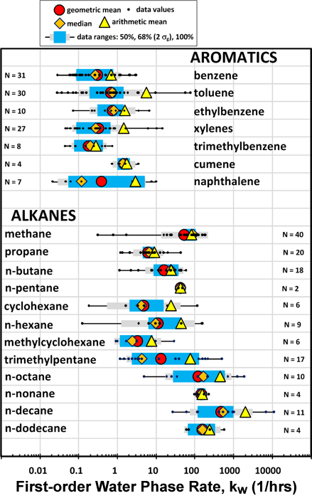
First-order water phase biodegradation rates (hr^-1) in aerobic vadose zone soils.

Source: DeVaull 2011.

Baseline Soil O₂ Respiration Rate

The baseline soil O₂ respiration accounts for the natural oxygen demand from the soil and may be specified directly or estimated from the soil organic carbon level (f_oc) based on an empirical relationship developed by DeVaull (2007), as follows:

Baseline Soil O₂ Respiration Rate = 1.69 (mg O₂/g_oc day) x f_oc

For the range 0.0004 < f_oc < 0.4, errors in the O₂ respiration estimate are within a factor of approximately 10 of the correlation at a 95% confidence level (DeVaull 2007). This equation is the BioVapor default value and is recommended in the absence of site-specific data.

Minimum O₂ for Aerobic Respiration

The BioVapor model default of 1% is reasonable for modeling purposes. Evidence from field studies with detailed profiles indicates O₂ depletion to low concentrations (<<1%) and a corresponding reduction in petroleum vapor concentrations (see, for instance, Davis, Patterson, and Trefry 2009).

Model Sensitivity

The BioVapor model can show a large sensitivity to source zone concentration and vertical separation distance in cases where biodegradation is the primary attenuation mechanism (DeVaull 2007; Weaver 2012). For these conditions, parameters relating to subsurface O₂ availability (O₂ concentration, foundation airflow), the biodegradation rate and soil moisture can have a significant influence on model estimates (Weaver 2012). Table 5-1 provides a qualitative evaluation of model sensitivity and uncertainty (and recommended data sources).

At sites where biodegradation is negligible, such as sites with high concentration sources and short vertical separation distances, the sensitivity of the BioVapor model is similar to that for the J&E model, which is applicable for nondegrading chemicals. For these conditions, parameters describing the building enclosure and foundation show a significant effect on model estimates (Weaver and Tillman 2005; Weaver 2012; Picone et al. 2012). These parameters include most significantly the building air exchange rate and the foundation air flow rate.

When using a PVI model such as BioVapor, conduct a sensitivity analysis by varying key input parameters to account for uncertainty and variability in site conditions. The key parameters affecting subsurface fate and transport include the O₂ boundary conditions, the first-order decay rate, the PHC source vapor strength, and the soil moisture content. Input a conservative estimate of the distance from the building foundation to the subsurface PHC source. Appendix I includes a more detailed discussion of parameter estimates and input values.